3 Corrections
This week is about image corrections, including geometric correction, atmospheric correction, relative correction, absolute correction, empirical line correction, orthorectification correction, mosaicking, texturing and PCA.
Code provided is in R.
3.1 Summary
3.2 Data Correction
Satellite data isn’t perfect, will have flaws and we need to fix it before we get into it, yuh.
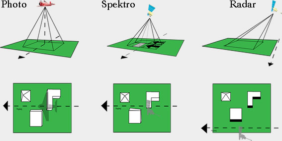
3.2.1 Geometric Correction
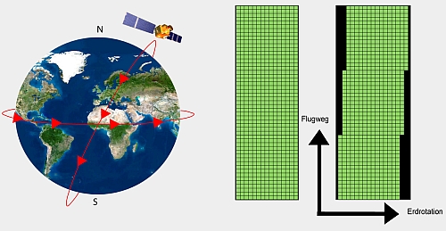
Process of removing geometric distortions caused by factors such as sensor perspective (off nadir), terrain relief (hill v flat ground), Wind (on plane) and Earth’s curvature and rotation.
Images:
3.2.1.1 Solution
Ground Control Points (GPS) to match satellite images to a reference datasets — another map, GPS data etc, using regression.
- Forward Mapping: we have the xy in a correct image, xiyi in the uncorrected data, and change the data to it.
- but the point is randomly placed on the correct image — not ideal
- Backward Mapping: predicting the wrong image with the correct image — more accurate, QGIS.
- takes every point of the correct image and maps it onto the uncorrected image
RMSE and Resampling
Normally RMSE is set as 0.5, but you might want to add more GCPs to reduce RMSE.
During this, data might be slightly shifted → so must resample the final raster by aligning via the nearest neighbour, linear, cubic. But grid cells might not align due to resolution etc etc.
3.2.2 Atmospheric Correction
3.2.2.1 Mainly scattering & topographic attenuation
Adjacency Effect: reflective surfaces bleeds into other pixels caused by scattering, making the image hazy and reduces contrast.
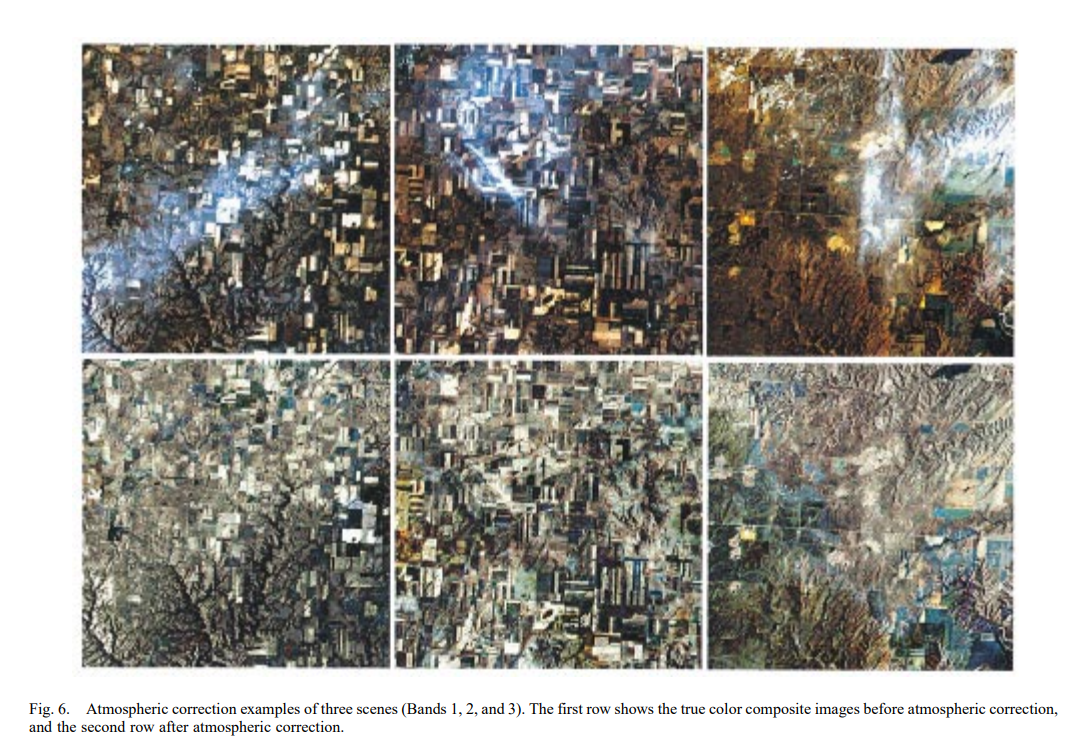 Image: Wang et al. (2012)
When and when not to correct:
| Unnecessary | Necessary |
|---|---|
| Classification of a single image | Biophysical parameters needed (e.g. temperature, leaf area index, NDVI) |
| Independent classification of multi date imagery | Using spectral signatures through time and space |
| Single dates data | |
| Already Composited images |
BUT : Andy corrects it all anyway, just in case
3.2.2.2 Solution
Relative Correction
Take a really dark pixel ( often the ocean) so that it can be assumed that it does not reflect the atmosphere at all, and subtract it to each pixel as a baseline.
Psuedo Invariant Features (PIF)
- from different images to identify features that don’t change (carparks)
- take regression, where y is the base image, apply model.
- base model often is the middle one in time series.
Absolute Correction
- Change digital brightness values into a scaled surface reflectance via atmospheric radiative transfer models. This is done to the whole image
- But this is difficult to do bc needs a lot of data and money.
Empirical Line Correction
- Go out to the field at take measurements using a field spectrometer, but you need to be at the right time a place where the satellite is right above…
- This is also essentially done through linear regression
3.2.3 Orthorectification Correction
Make things nadir. This would be used if satellite passes adjacent to a mountain top instead of directly above it.
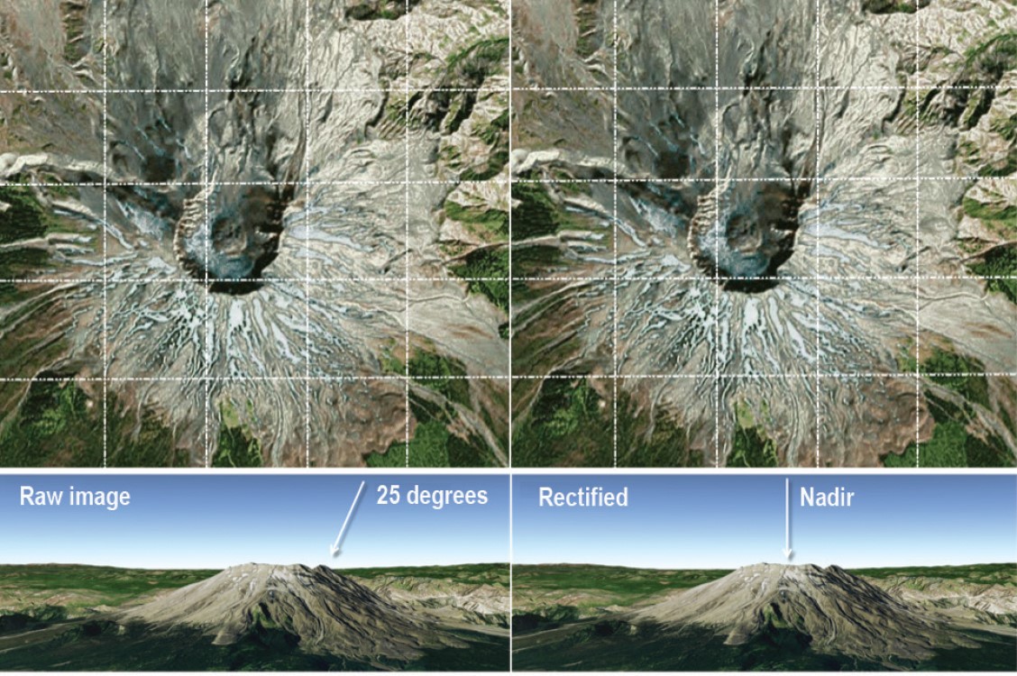
Often uses cosine correction to calculate sun’s zenith and incidence angle
3.2.4 Radiometric Calibration
Satellites capture image brightness and is stored as Digital Number, which has no units and difficult to use!
Radiometric Calibration is converting DN to spectral radiance.
After all of that…
There is Landsat ARD - surface reflectance that is already corrected…
But it’s good to know anyway and not all data are ARD (drone images, v high resolution images)
3.3 Data Joining
3.3.1 Mosaicking
Says what it does on the can! Just like feathering and merging, we are joining 2 or more images together.
The images must have some overlapping, or else there’ll be gaps in your map. The overlapping will be dealt with through feathering (blending) so that seamlines are not visible.
Merging code:
m1 <- terra::mosaic(listlandsat_9i, listlandsat_9ii, fun="mean")3.4 Image Enhancement
To emphasize/exaggerate certain spectral traits. ### Contrast Enhancement
Different materials don’t reflect varying energy back — making it hard to differentiate between things. Images are also designed to avoid saturation in DN.
- Image stretching applied to DN
3.4.1 Ratio
Difference between 2 spectral bands that have a certain spectral response – making it easier to identify certain landscape features. This is the remote sensing index, index that refers to a specific item, and uses simple formula to get them.
Refer to Index Database for more!! There is an index for virtually everything on earth. From soil type, tree health, moisture level, rock/metal type etc etc…
Here we’re extracting healthy vegetation, formula from Normalized Difference Vegetation Index. Band 5 - Band 4 (red)
m1_NDVI <- (m1$LC09_L2SP_137043_20230126_20230128_02_T1_SR_B5 - m1$LC09_L2SP_137043_20230126_20230128_02_T1_SR_B4 ) / (m1$LC09_L2SP_137043_20230126_20230128_02_T1_SR_B5 + m1$LC09_L2SP_137043_20230126_20230128_02_T1_SR_B4)

m1_NDVI %>%
  plot(.)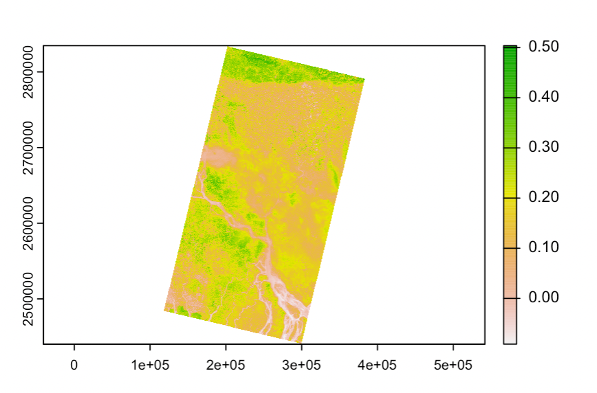
The greener, there more healthy vegetation there is. Since this is EO image of Dhaka (aka flood zone), vegetation is only present further to the north.
This is to filter out features that has higher NDVI score.
veg <- m1_NDVI %>%
  terra::classify(., cbind(-Inf, 0.2, NA))
3.4.2 Filtering
Filtering refers to any kind of moving window operation (zooming out) to our data, saved as a separate raster file, either low or high pass filters.
3.4.3 Texture
Use glcm package to select 8 texture measures.
- Can specify size of moving window here
- specify shift in co-occurency — if there are multiple shifts — will return mean for each pixel.
This will take 7-10mins!!
glcm <- glcm(band4_raster,
                   window = c(7, 7),
                   #shift=list(c(0,1), c(1,1), c(1,0), c(1,-1)),
                   statistics = c("homogeneity"))
INSERT CODE
3.4.4 Data Fusion
append new raster data onto existing data OR merge several bands and make new easter dataset
Here: merging the texture measure (glcm) and the original raster
# for the next step of PCA we need to keep this in a raster (and not terra) format...
m1_raster <- stack(m1)

Fuse <- stack(m1_raster, glcm)
3.4.5 PCA
reduce dimensionality of data!
To scale data, aka compare data that isnt measured in the same way (spectral bands 4 and 5) and textural data - use the scale function to standardise deviation.
To get the mean: use scale = FALSE We can also set the number of samples for PCA
library(RStoolbox)

Fuse_3_bands <- stack(Fuse$LC09_L2SP_137043_20230126_20230128_02_T1_SR_B4, Fuse$LC09_L2SP_137043_20230126_20230128_02_T1_SR_B5, Fuse$glcm_homogeneity)

scale_fuse<-scale(Fuse_3_bands)

pca <- rasterPCA(Fuse,
                 nSamples =100,
                 spca = TRUE)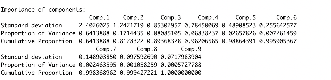
Here Comp 1 & 2 explains 0.81% of the variance. Often this is enough for analysis, so we extract only these 2.
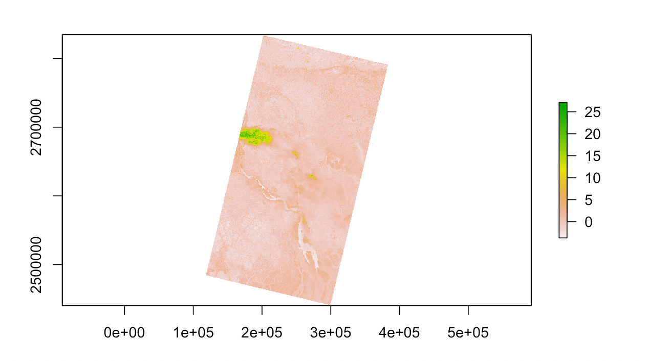
This is the output of just layer 1.
3.5 A little about data format
Landsat data are collected in rows and paths made up of grids of images.
Data is are in tiers and levels.
Tier: Tier 1 denotes best quality, Tier 2 are good but with some clouds that affects radiometric calibration, covering GCPs.
Level: Level 1 is delivered through DN, Level 2 has surface reflectance and surface temperature, Level 3 are specific products ie Burned Area, surface water extent.
3.6 Application
We outlined generally how these corrections and enhancements are executed. However when it comes to application, there are lots of debates around how best to correct/enhance an image.
For example, Wang et al. (2012) found we choose and design the Ground Control Points (GCPs) have strong effects on the accuracy of geometric correction. They used a universal kriging model-based sampling method that takes into account the spatial auto-covariance of regression residual, and extracts results accordingly. They found that the more disperse and even the distribution of the GCPs, the higher the geometric correction precision.
Academics also develop new methods of correction and enhancements specifically to extract earth features they want and accessibility of certain methods. Pandey, Tate, and Balzter (2014) use PCA to map tree species in coastal Portugal depending on the tree species’ reflectance signatures. He highlighted the high cost involved to do this using GCPs, and that the increasing temporal and spectral frequency of earth data made developing automatic image registration software possible. At the end 15 PC layers contained 99.42% of the information of the original hyperspectral image.
Sometimes you don’t know if an image needs to be corrected or not if there are no obvious signs of haze or clouds visible to us. In a similar vein to reduce costly ground observation data (but also to test whether atmospheric correction (AC) is needed for improving the reliability of the estimated values of 2 key clear water parameters), Sriwongsitanon, Surakit, and Thianpopirug (2011) evaluated the influence of atmospheric correction and number of sampling points on the accuracy of water clarity assessment. They collected data on clarity and sediment parameters at 80 ground observation points as reference and used three Landsat 5 TM images to conduct the experiment in the largest lake in Thailand. They found AC has a statistically significant influence over the max and min values of the sediment parameter and clarity parameter, making the images more accurate in assessing water clarity, thus encouraged to be applied to when assessing clarity of water. They also concluded that only 32/80 of the observation points were needed for the satellite image to obtain a reliable assessment as a result of AC, instead of all 80. (wohoo!)
3.7 Reflection
Understanding how satellite images are tweaked and handled before they could actually be used for analysis feels the same as data cleaning before we go into EDA. Although cumbersome at times, I feel this is the most effective way to get to know data before conducting analysis. It’s also generally good practice to understand how values are generated through by calculating them step by step, rather than just one line of code provided by a package. We will eventually encounter data that isn’t corrected. It’s good to at least to know generally how to approach correction. I’m also looking forward to GEE and see how the platform streamlines the process.
The possibilities with Earth Observation data seems to be… endless? Essentially anything activities larger than 10 by 10m can be detected on satellite images. That thought in itself is quite overwhelming, because when you can do everything, where do you start?
It’s been very useful to know how these correction and enhancement methods work before we dive straight into GEE with ARD. Surprisingly I didn’t find this week’s content that overwhelming (compared to week 7, just you wait). In contrast I really felt it laid the necessary foundation for me to understand how one would process earth observation data. I feel more confident knowing how to deal with earth observation data, in case I ever need to deal with raw images.