6 Classification I
Week 6 is about classification! When we get an image from satellites, we need the programme to be able to identify types of land cover for masses of data. While we can’t do this manually, we need to rely on Machine Learning methods.
From this point onwards I am going to focus on explaining the concepts and understanding the methods instead of codes. I want to spend this time to make sure I really understand ML and classification methods before I execute codes.
6.1 Summary
6.1.1 Introduction to Machine Learning
Machine Learning is the science of computer modelling of learning process.
Machine learning models use a type of inductive inference where the knowledge base (rule of thumbs) are learned from specific historical example (the training data), and these general conclusion to predict future.
6.1.1.1 Classification & Regression Trees (CART): Classification
Classification Trees
When a decision tree classify things to categories.
Classify data into 2+ discrete categories, split into further branches until all categories of decision have been made.
A good classification tree should be multi layered because just one independent vary would often result in impure results (where the predictive power of the independent variable is not 100% accurate)
The more relevant dependent variables in the tree, the less impure the result should be, and the stronger the predictive accuracy.
How do we know what order we put our dependent variables in the classification tree?
We calculate a Gini Impurity for each variable, and the one with the lowest impurity becomes the root.
we dont expect the leaves from the root node to be pure, so we calculate the the Gini impurity of the remaining variables, and choose the variable with the lowest Gini impurity score, split the node and so on, until nodes become leaves.
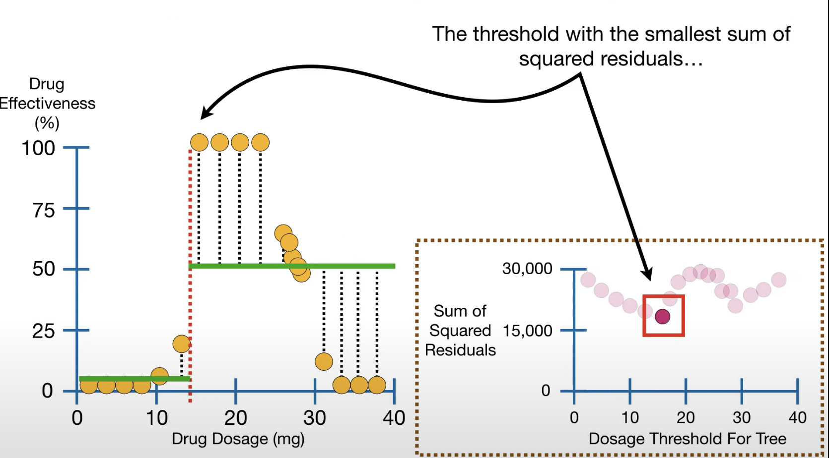
Regression Trees
When decision tree predicts numeric, continuous discrete values
When linear 1 relationship does not fit data, we split the data into smaller subset, and run several different regressions for each chunk
How do we know where to cut?
- Sections are divided based on thresholds (nodes) and the SSR (Sum of Square Residuals) is calculated.
- Again, ones with lowest SSR becomes the root, and so on.
- Outcome: each leaf should represent the value that is close to the data
Source: StatQuest with Josh Starmer (2018)
Public Enemy: Overfittiing
Subsetting and dividing dataset too much could lead to overfitting — meaning the model is so fine tuned to the detail on the dataset it is learning from, it is unable to effectively predict outcome with a different dataset.
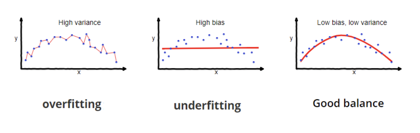
Bias: difference between predicted value and true value — bad a being precise
Variance: variability of model for a given point — bad a generalising
You want a bit of both!
Preventative measures:
Limit how the tree grows – set minimum of at least 20pixel per leaf
Weakest Link pruning:

Image: The formidable Anne Robinson
Calculate SSR for each tree. From no leaf removal to more leaves removal
It is expected that as more leaves are removed, the SSR gets bigger. The point is so that the model doesn’t fit the training data too well anyway.
With each tree’s SSR, we calculate the Tree Score (the lower the better).
Tree Score = SSR + αT
T = number of leaves
α = tree penalty. The more leaves removed, the higher the α.
How to decide on α?
Build a full size (training and testing) regression tree, where α becomes 0, where tree score is the lowest. Repeat and get a different α values for each tree.
- Return to the training data, and apply α values from before, which dictates where the data is split
Do this process 10 times for cross validation — the value of α that gives the smallest ~SSR is the final value → select the tree that used the full data with that specific alpha
6.1.2 Random Forest
Many decision trees from 1 set of data.
Decision trees on their own are pretty inaccurate, not flexible when classifying new samples. Random Forests are simple, but also very adaptable when met with new data, improving accuracy
Validation data: different from OOB, not in the original dataset at all.
Bootstrapping: Where you randomly select samples, and you’re allowed to pick the same sample more than once.
6.1.3 Image Classification
Okay, so how do we apply what we learned above onto image classification, and how do they relate?
6.2 Application
Examples of image classification
Support Vector Machine & Maximum Likelihood: which is better?
Otukei and Blaschke (2010) explored and compared Decision Trees, Support Vector Machines and Maximum Likelihood techniques when it comes to classifying land cover change in Uganda . They highlighted that expert knowledge is essential in creating the thresholds and boundaries when building analysis, but this is often lacking in the Global South. They proposed to use data mining approaches to determine decision threshold for these analyses.
Uganda has undergone huge land cover changes, where wetlands have been converted to crop fields to support livelihoods. The was conducted to evaluate the land cover change that has happened between 1981 and 2001.
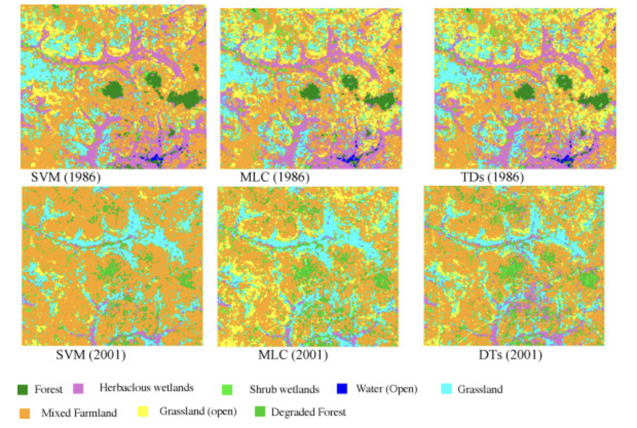
Above you can see the classification outputs for each methods. All 3 methods performed well with accuracies above 85%, with decision trees performing slightly better with overall accuracy of 93%.
It is important to note however, each classification methods has it’s pros and cons. Often which method you choose to use depends on the nature of your data and what output you are looking for. And sometimes, it might be down to the overall accuracy to decide.
For complex systems, non parametric approaches are often more flexible and data driven as they do not require any assumptions or mathematical models about the underlying probability distribution of your data.
Within more well researched fields, such as LULC and vegetation classification, Maximum Likehood tends to be more popular as there are often clear distinction between different feature classes.
6.2.0.1 Monitoring invasive species using SVM
Gavier-Pizarro et al. (2012) did a really interesting and novel project using Landsat TM/ETM+ data and SVM to monitor the invasion of the Chinese tree glossy privet that is aggressively replacing native forests in Argentina, causing huge cause of concern regarding conservation. SVM was chosen simply because this approach has been proven to be effective in vegetation classification.
Landsat TM/ETM+ data are only at 30m resolution, but these images have been successful in mapping invasion for single points in time that forms homogeneous patches larger than 0.5 hectares, given surround phenology of native species are different. Glossy Privets are much lower in luminosity compared to native vegetation.
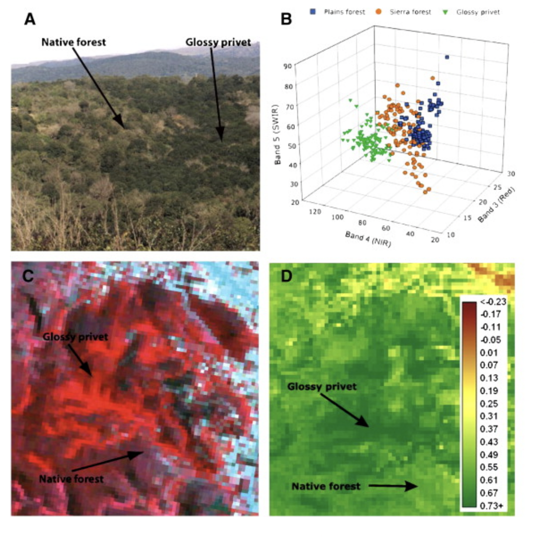
Source: Gavier-Pizarro et al. (2012)
Since the classes are not linearly separable, a Gaussian kernal function was applied to gain the optimal values of C and gamma for SVM. These parameters were then used to classify the multitemporal stacks of Landsat images to map glossy privet invasion.
I find this technique of mapping single points in time to overcome the problem of low spatial resolution very interesting. The authors did not mention if this approach has reduced the overall accuracy either. Another problem with is approach is that the spread of invasive species has to be quite prominent already for detection to occur. The study highlighted areas of mixed species/early stages were classified as native forest. This this analysis only allows for a reactive measure against the invasive expansion.
6.3 Reflection
This week we looked into the early days methods of classification, first diving into the concept of decision trees and random forests. These methods are very intuitive to me. I visualise this as a person walks down the street and decide if they want to go left or right at a junction. A path is then paved depending on the characteristics of the person: their ethnicity, social class, how they’re feeling that day.
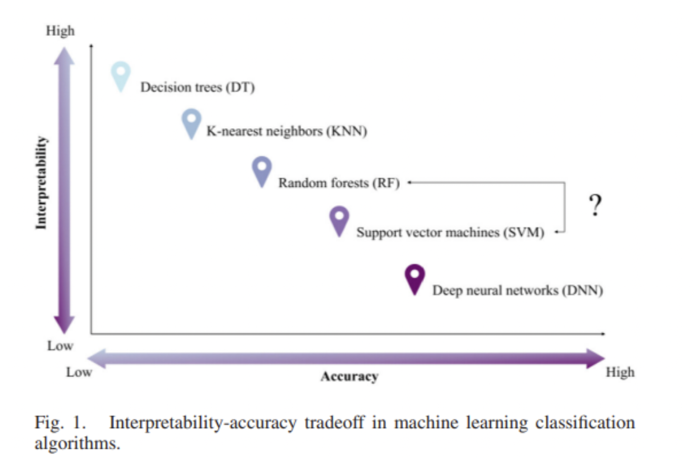
Andy ended this week’s lecture highlighting the accuracy and interpretability trade off between different classification methods. Coming from a social science background, I would intuitively choose a classifier that is easier to understand. My approach to data science is that insights gains are ultimately generated to inform policy making. The problem of the blackbox is concerning because when stakeholders, clients and even data scientists themselves don’t entirely understand how these insights are generated, this threaten the trustworthiness of this insight. I think as machine learning and deep learning continue to advance rapidly, increasing interpretability needs to be prioritised. Because utimately, data isn’t always correct. And if we don’t know how insights came to be, we wouldn’t know what went wrong and how we would fix it.